Formulas for the basic waveforms

In the following formulas, the variables are :

• $t$ : time, represented in the x-axis
• $a$ : amplitude
• $f$: frequency
• $p$: period = $1/f$

We start by importing the numpy and matplotlib packages and defining some variables :

import matplotlib.pyplot as pp
import numpy as np

f = 1            # [Hz]
p = 1/f          # period in [s]
a = 3            # amplitude; full peak-to-peak will be 2*amplitude
periods = 2      # show 2 periods
samples = 1000   # sample points (resolution of the graph)

t = np.linspace(0, periods/f, samples)    # Return evenly spaced numbers over a specified interval

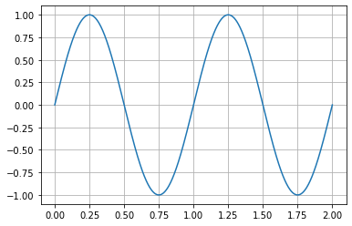
Sine wave

$\large y(t)=a\sin(2\pi ft)$

pp.plot(t, a * np.sin(2 * np.pi * f * t))
pp.grid()

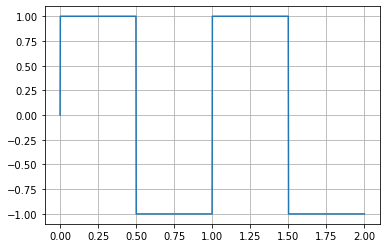
Square wave

$\large y(t)=a\operatorname {sgn}(\sin 2\pi ft)$

pp.plot(t, a * np.sign(np.sin(2 * np.pi * f * t)))
pp.grid()

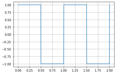
alternative with the floor function :

$\large x(t)=a(2\left(2\lfloor ft\rfloor -\lfloor 2ft\rfloor \right)+1)$

pp.plot(t, a * (2 * (2*np.floor(f * t) - np.floor(2 * f * t)) + 1))
pp.grid()

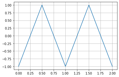
Triangle wave

$\large y(t) = \frac{4a}{p} \left| \left( \left(t - \frac{p}{4}\right) \bmod p \right) - \frac{p}{2} \right| - a$

pp.plot(t, a * abs(((t-p/4) % p) - (p/2)) * 4 / p - a)
# '%' can be replaced by the numpy mod function :
# amplitude * abs(np.mod((t-T/4), T) - (T/2)) * 4 / T - amplitude
pp.grid()

alternative as the absolute value of a shifted sawtooth wave :

$\large y(t)=a(4\left|{\frac {t}{p}}-\left\lfloor {\frac {t}{p}}+{\frac {1}{2}}\right\rfloor \right|-1) = a(4\left|ft-\left\lfloor ft+{\frac {1}{2}}\right\rfloor \right|-1)$

pp.plot(t, a * (4 * abs(f * t - np.floor(f * t + 1/2)) - 1))
pp.grid()

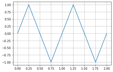
if we correct the phase offset :

$\large y(t)=a(4\left|f(t+{\frac {1}{4}})-\left\lfloor f(t+{\frac {1}{4}})+{\frac {1}{2}}\right\rfloor \right|-1)$

pp.plot(t, a * (4 * abs(f * (t+1/4) - np.floor(f * (t+1/4) + 1/2)) - 1))
pp.grid()

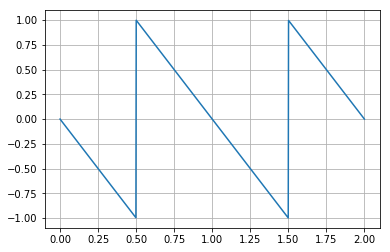
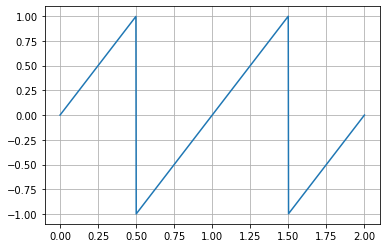
Sawtooth wave

$\large 2a\left({\frac {t}{p}}-\left\lfloor {\frac {t}{p}}+{\frac {1}{2}}\right\rfloor \right) = 2a\left(ft-\left\lfloor ft+{\frac {1}{2}}\right\rfloor \right)$

pp.plot(t, a * 2 * (f * t - np.floor(f * t + 1/2)))
pp.grid()

Inverse sawtooth

$\large 2a( \left\lfloor ft-{\frac {1}{2}}\right\rfloor - ft + 1)$

pp.plot(t, 2 * a * (np.floor(f * t - 1/2) - f * t + 1))
pp.grid()