Low-Pass Filter on a Squarewave

A square wave is rich in odd harmonics, its spectrum contains the fundamental frequency plus components at $3 f$ , $5 f$ , $7 f$ , $\dots$ with amplitudes decreasing as $1/ n$ . Passing it through a low-pass RC filter progressively attenuates those harmonics, rounding the sharp edges and making the waveform increasingly sine-like as the cutoff frequency drops. This is a useful exercise for understanding filter behaviour, and also a practical technique: a PWM output from a microcontroller can be converted to an analogue voltage using nothing more than a resistor and a capacitor.

In this notebook, the square wave is set to $f = 50 Hz$ . The RC filter is defined with $R = 1 k Ω$ and $C = 1 μ F$ , giving a cutoff frequency of $f_{c} \approx 159.15 Hz$ , about three times the signal frequency. The filter is then also tested with $C /10$ ( $f_{c} \approx 1591 Hz$ , well above the signal) and $C \times 10$ ( $f_{c} \approx 15.9 Hz$ , below the signal) to illustrate the range of effects.

Transfer function of the RC low-pass filter

The output voltage is derived from the voltage divider formed by $Z_{R} = R$ and $Z_{C} = 1/ j ω C$ :

V_{o u t} (t) = V_{in} (t) (\frac{Z _{C}}{Z _{R} + Z _{C}}) = V_{in} (t) (\frac{- j / ω C}{R - j / ω C}) = V_{in} (t) (\frac{1}{j R ω C + 1})

import matplotlib.pyplot as plt
import numpy as np

def rc_low_pass_filter(f, R, C):
    omega = 2*np.pi*f
    return 1.0/(1j*R*omega*C+1.0)

Cutoff frequency

The cutoff frequency $f_{c}$ is defined by:

f_{c} = \frac{1}{2 π R C}

At $f_{c}$ , the filter attenuates the signal by $- 3 dB$ , meaning the output amplitude drops to $1/ 2 \approx 70.7%$ of the input. Above $f_{c}$ the attenuation increases at $- 20 dB$ per decade (i.e. a ×10 increase in frequency halves the output amplitude again).

def rc_low_pass_cutoff(R, C):
    return 1.0/(2*np.pi*R*C)

Define the filter

R=1.0e3    # 1kOhm
C=1.0e-6   # 1µF

fc = rc_low_pass_cutoff(R, C)

print("Filter cut off is: {:7.2f} Hz".format(fc))

Filter cut off is: 159.15 Hz

Define the square wave

f = 50Hz

from scipy import signal

# Frequency of the square wave :
f = 50.0   # frequency in [Hz]
T = 1.0/f  # period of the signal in [s]

# Sample points :
samples = 2**15                     # a 2^N number of samples makes the FFT very fast
periods = 2                         # number of periods to show
delta_t = T * periods / samples     # time corresponding to one sample

t = np.linspace(0, 1/f * periods, samples, endpoint=False)

y = signal.square(2*np.pi*t*f)     # square wave, amplitude ±1 V, peak-to-peak = 2 V

plt.figure(figsize=(10,5))
plt.plot(1e3*t, y)             # Change the x-axis scale to ms by multiplying by 10^3
ax = plt.gca()
plt.grid(True)
plt.title("Square Wave")
plt.xlabel("time(ms)",position=(0.95,1))
plt.ylabel("signal(V)",position=(1,0.9))
plt.show()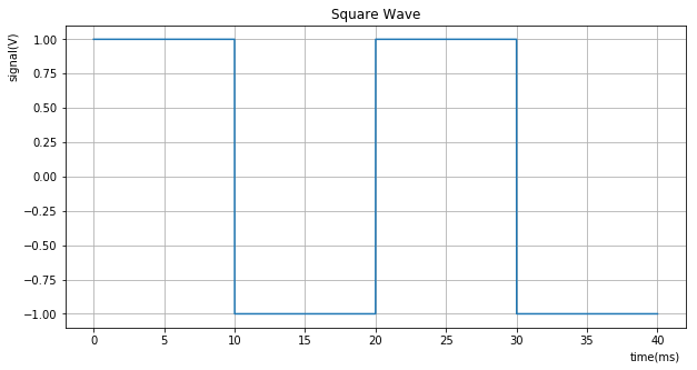

Apply the filter to the square wave

The filter is applied in the frequency domain: the FFT of the square wave is multiplied bin-by-bin by the complex filter gain $H (f)$ , then transformed back with an IFFT. This is mathematically equivalent to convolution in the time domain but far more efficient for long signals.

from scipy.fftpack import fft, ifft, fftfreq, fftshift

# helper function :
def apply_filter_and_plot(R, C, samples, delta_t, y):
    y_out = ifft(fft(y) * rc_low_pass_filter(fftfreq(samples, delta_t), R, C))
    plt.figure(figsize=(10,5))
    plt.plot(1e3*t,np.real(y_out))
    ax = plt.gca()
    plt.grid(True)
    plt.title("Square wave with LP filter. R={:7.2f} Ohms, C={:0.2f} uF, cutoff={:0.1f} Hz".format(R, C*1e6, rc_low_pass_cutoff(R, C)))
    plt.xlabel("time(ms)",position=(0.95,1))
    plt.ylabel("signal(V)",position=(1,0.9))
    plt.show()

$f_{c} = 159 Hz$ , approximately $3 \times$ the signal frequency ( $C = 1 μ F$ ). The cutoff is close to the 3rd harmonic ( $150 Hz$ ), so the higher harmonics are significantly attenuated and the edges begin to round noticeably.

apply_filter_and_plot(R, C, samples, delta_t, y)

Square wave filtered at fc ≈ 159 Hz (C = 1µF)

$f_{c} = 1591 Hz$ , well above the signal frequency ( $C = 0.1 μ F$ ). The cutoff is far above the fundamental and most audible harmonics, so the filter has little effect and the square wave is largely preserved.

apply_filter_and_plot(R, C/10, samples, delta_t, y)

Square wave filtered at fc ≈ 1591 Hz (C = 0.1µF)

$f_{c} = 15.9 Hz$ , below the signal frequency ( $C = 10 μ F$ ). The cutoff is now below the fundamental itself, so even the first harmonic is attenuated. The output is nearly sinusoidal, only the fundamental survives with meaningful amplitude.

apply_filter_and_plot(R, C*10, samples, delta_t, y)

Square wave filtered at fc ≈ 15.9 Hz (C = 10µF)

Low-Pass Filter on a Squarewave

Transfer function of the RC low-pass filter

Cutoff frequency

Define the filter

Define the square wave

Apply the filter to the square wave

See also