High-Pass Filter on a Squarewave
Where a low-pass filter removes high-frequency harmonics and rounds the edges of a square wave, a high-pass filter does the opposite: it blocks the low-frequency content, including the DC component and the fundamental, and passes only the rapid transitions. Applied to a square wave, it produces a characteristic spike or “differentiated” shape at each edge, with the signal decaying back toward zero between transitions.
Transfer function of the RC high-pass filter
The output is taken across rather than , which is the complement of the low-pass case:
import matplotlib.pyplot as plt
import numpy as np

def rc_high_pass_filter(f, R, C):
    omega = 2*np.pi*f
    return 1j*R*omega*C / (1.0 + 1j*R*omega*C)
Cutoff frequency
The cutoff frequency is the same expression as for the low-pass filter:
At , the filter attenuates the signal by (output amplitude of input). Below the attenuation increases at per decade as frequency decreases.
def rc_high_pass_cutoff(R, C):
    return 1.0/(2*np.pi*R*C)
Define the filter
R=1.0e3    # 1kOhm
C=1.0e-6   # 1µF

fc = rc_high_pass_cutoff(R, C)

print("Filter cut off is: {:7.2f} Hz".format(fc))
Filter cut off is: 159.15 Hz
Define the square wave
f = 50Hz
from scipy import signal

# Frequency of the square wave :
f = 50.0   # frequency in [Hz]
T = 1.0/f  # period of the signal in [s]

# Sample points :
samples = 2**15                     # a 2^N number of samples makes the FFT very fast
periods = 2                         # number of periods to show
delta_t = T * periods / samples     # time corresponding to one sample

t = np.linspace(0, 1/f * periods, samples, endpoint=False)

y = signal.square(2*np.pi*t*f)     # square wave, amplitude ±1 V, peak-to-peak = 2 V

plt.figure(figsize=(10,5))
plt.plot(1e3*t, y)                  # x-axis in ms
ax = plt.gca()
plt.grid(True)
plt.title("Square Wave")
plt.xlabel("time(ms)",position=(0.95,1))
plt.ylabel("signal(V)",position=(1,0.9))
plt.show()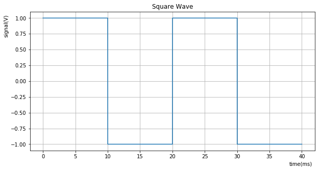
Apply the filter to the square wave
The filter is applied in the frequency domain: the FFT of the square wave is multiplied bin-by-bin by the complex filter gain , then transformed back with an IFFT. This is mathematically equivalent to convolution in the time domain but far more efficient for long signals.
from scipy.fftpack import fft, ifft, fftfreq, fftshift

# helper function :
def apply_filter_and_plot(R, C, samples, delta_t, y):
    y_out = ifft(fft(y) * rc_high_pass_filter(fftfreq(samples, delta_t), R, C))
    plt.figure(figsize=(10,5))
    plt.plot(1e3*t,np.real(y_out))
    ax = plt.gca()
    plt.grid(True)
    plt.title("Square wave with HP filter. R={:7.2f} Ohms, C={:0.2f} uF, cutoff={:0.1f} Hz".format(R, C*1e6, rc_high_pass_cutoff(R, C)))
    plt.xlabel("time(ms)",position=(0.95,1))
    plt.ylabel("signal(V)",position=(1,0.9))
plt.show(), approximately the signal frequency (). The cutoff is above the fundamental (), so the fundamental and lower harmonics are significantly attenuated. The output shows clear spikes at each transition with visible exponential decay in between, the classic differentiator behaviour.
apply_filter_and_plot(R, C, samples, delta_t, y)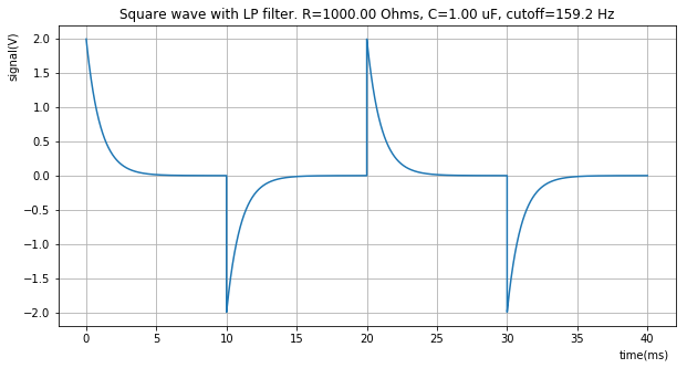
, well above the signal frequency (). The cutoff is now far above the fundamental and all significant harmonics, so almost all the signal content is attenuated. The output is nearly zero with only very faint spikes at the transitions.
apply_filter_and_plot(R, C/10, samples, delta_t, y)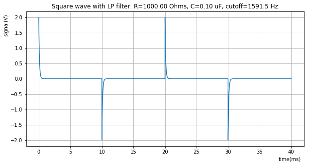
, below the signal frequency (). The cutoff is now below the fundamental, so all harmonics pass with relatively little attenuation. The output closely resembles the original square wave, though the DC component is fully removed and there is a slight droop on the flat portions due to residual high-pass effect near the fundamental.
apply_filter_and_plot(R, C*10, samples, delta_t, y)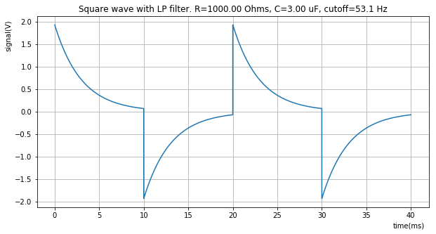
See also:
- Formulas for the basic waveforms
- Effect of an RC low-pass filter on a squarewave.
- More info about RC high-pass filters: https://www.electronics-tutorials.ws/filter/filter_3.html
- Inspiration for this notebook: https://notebook.community/mholtrop/Phys605/Python/Signal/RC_Filters_in_Python